Question

How does social isolation during a critical development period affect the behavior of hooded rats? Psychology students assigned 24 young female rats at random to either isolated or group housing, then similarly assigned 24 young male rats. This is a randomized block design with the gender of the 48 rats as the blocking variable and housing type as the treatment. Later, the students observed the time that a rat spends in object play during an observation period. The file ??26‑30.??? records the time (in seconds) that each rat devoted to object play.

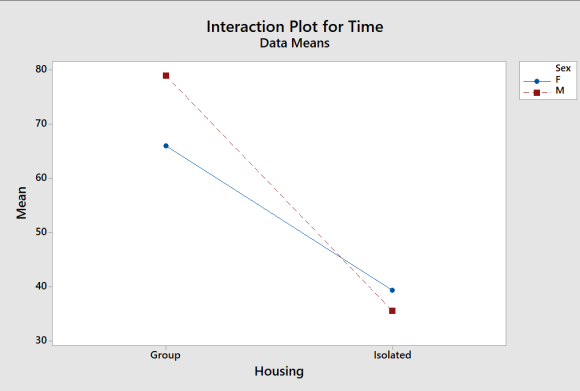
(a) Using the software of your choice, make a plot of the 4 group means by calculating the values for the table.

	Gender
	M	F
Isolated	?	?
Group	?	?

Animal	Sex	Housing	Time
1	M	Isolated	29
2	M	Isolated	34
3	M	Isolated	35
4	M	Isolated	20
5	M	Isolated	34
6	M	Isolated	24
7	M	Isolated	26
8	M	Isolated	36
9	M	Isolated	74
10	M	Isolated	9
11	M	Isolated	49
12	M	Isolated	57
13	F	Isolated	37
14	F	Isolated	8
15	F	Isolated	30
16	F	Isolated	49
17	F	Isolated	15
18	F	Isolated	69
19	F	Isolated	36
20	F	Isolated	36
21	F	Isolated	38
22	F	Isolated	44
23	F	Isolated	51
24	F	Isolated	59
25	M	Group	123
26	M	Group	121
27	M	Group	109
28	M	Group	126
29	M	Group	38
30	M	Group	55
31	M	Group	3
32	M	Group	78
33	M	Group	73
34	M	Group	70
35	M	Group	39
36	M	Group	113
37	F	Group	94
38	F	Group	10
39	F	Group	149
40	F	Group	54
41	F	Group	78
42	F	Group	72
43	F	Group	80
44	F	Group	101
45	F	Group	69
46	F	Group	46
47	F	Group	13
48	F	Group	26

Calculate the values ?‑? to fill in the table. (Enter your answer rounded to two decimal places for ? and ? .)

?=

?=

(Enter your answer rounded to one decimal place for ? and ? .)

?=

?=

Is there a large interaction between gender and housing type? Which main effect appears to be more important?

The means plot suggests a strong main effect for housing and a possible (weak) interaction.

The means plot suggests a weak main effect for housing and a possible (weak) interaction.

The means plot suggests a strong main effect for housing and a strong interaction.

The means plot suggests a strong main effect for isolated and a possible (weak) interaction.

(b) Verify that the conditions for ANOVA inference are satisfied.

The standard deviations vary from 17.08 to 40.1 , which gives a ratio slightly less than 2 . Dotplots show some outliers in the group housing distributions. We proceed with caution.

The standard deviations vary from 17.08 to 40.1 , which gives a ratio slightly greater than 2 . Dotplots show some outliers in the group housing distributions. We proceed with caution.

The standard deviations vary from 17.08 to 40.1 , which gives a ratio slightly less than 2 . Dotplots show some outliers in the isolated distributions. We proceed with caution.

The standard deviations vary from 17.08 to 40.1 , which gives a ratio much greater than 2 . Dotplots show some outliers in the group housing distributions. We proceed with confidence.

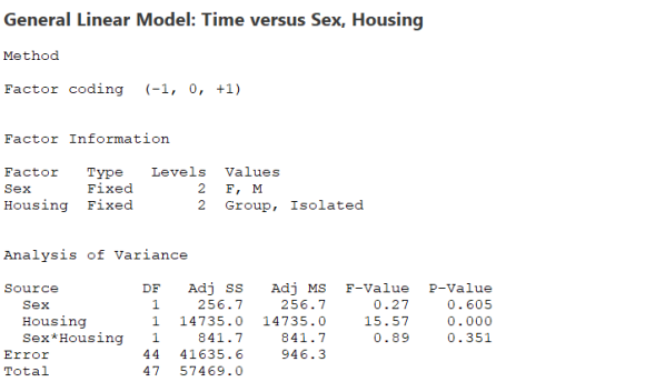
(c) Using the software of your choice find the complete two‑way ANOVA table. What are the ? statistics and ?‑values for interaction and the two main effects?

Find the ?‑values for housing, sex, and interaction. (Enter your answer rounded to four decimal places.)

?ℎ??????=

????=

????????????=

Find the ? statistics for housing. (Enter your answers rounded to two decimal places.)

?ℎ??????=

Find the ? statistics for sex, and interaction. (Enter your answers rounded to three decimal places.)

????=

????????????=

Select the best explanation as to why the test results confirm the tentative conclusions you drew from the plot of means.

The ANOVA table shows a significant effect of housing and sex. Interaction is not significant. This is consistent with the conclusions from the means plot.

The ANOVA table shows a significant effect of housing. Sex and interaction are not significant. This is consistent with the conclusions from the means plot.

The ANOVA table shows a significant effect of housing. Sex and interaction are not significant. This is not consistent with the conclusions from the means plot.

The ANOVA table shows a significant effect of Sex. Housing and interaction are not significant. This is consistent with the conclusions from the means plot.

Answer 1

Using Minitab

ByVar1   ByVar2   Mean1
F    Group    66.0000
F    Isolated    39.3333
M    Group    79.0000
M    Isolated    35.5833

means for each pair are above

Housing is significant , Sex and interaction are not significant