Question

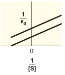
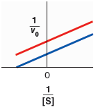
Below are shown three Lineweaver-Burk plots for enzyme reactions that have been carried out in the presence, or absence, of an inhibitor.

Part A

Indicate what type of inhibition is predicted based on Lineweaver-Burk plot.

	mixed inhibition
	competitive inhibition
	uncompetitive inhibition

 

Part B

Indicate which line corresponds to the reaction without inhibitor and which line corresponds to the reaction with inhibitor present.

	red - without inhibitor, blue - with inhibitor
	blue - without inhibitor, red - with inhibitor

 

Part C

Indicate what type of inhibition is predicted based on Lineweaver-Burk plot.

	mixed inhibition
	competitive inhibition
	uncompetitive inhibition

 

Part D

Indicate which line corresponds to the reaction without inhibitor and which line corresponds to the reaction with inhibitor present.

Indicate which line corresponds to the reaction without inhibitor and which line corresponds to the reaction

	blue - without inhibitor, red - with inhibitor
	red - without inhibitor, blue - with inhibitor

 

Part E

Indicate what type of inhibition is predicted based on Lineweaver-Burk plot.

	mixed inhibition
	competitive inhibition
	uncompetitive inhibition

 

Part F

Indicate which line corresponds to the reaction without inhibitor and which line corresponds to the reaction with inhibitor present.

	blue - without inhibitor, red - with inhibitor
	red - without inhibitor, blue - with inhibitor

Answer 1

Part-A

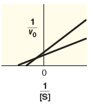
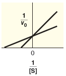
The lineweaver-Burk equation for the mixed inhibition is, \(\frac{1}{v_{0}}=\left(\frac{\alpha K_{m}}{V_{\max }}\right) \frac{1}{[s]}+\frac{\alpha^{\prime}}{V_{\max }}\)

Here, \(v_{0}\) is the initial velocity, \([s]\) is the substrate concentration,

$$ \alpha^{\prime}=\left(1+\frac{[\mathrm{I}]}{K_{I}^{\prime}}\right), \alpha=\left(1+\frac{[\mathrm{I}]}{K_{I}}\right) $$

\([\mathrm{I}]\) is the inhibitor concnetration, \(V_{\max }\) is the maximum velocity \(K_{I}^{\prime}\) and \(K_{I}^{\prime}\) are the dissociation constants, and \(K_{m}\) is the Michael's constant.

The corresponding lineweaver-Burk plot for the mixed inhibition is shown below:

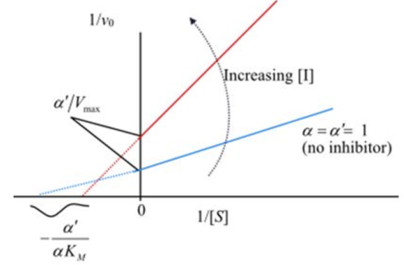
Plot 1: Lineweaver-Burk plot in the presence of mixed inhibitor

The curled arrow which is in anti-clock wise direction indicates increasing inhibitor concentration.

Compare the specified plot with the plot-1. Thus, based on the plot the enzyme reaction is a mixed inhibition type.

 

Part-B

Compare the specified plot with plot-1, Thus, the blue line indicates the line equation without inhibitor and, the red line indicates the line equation with inhibitor.

 

Part-C

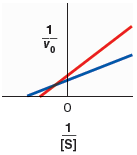
The lineweaver-Burk equation for the competitive inhibition is, \(\frac{1}{v_{0}}=\left(\frac{\alpha K_{m}}{V_{\max }}\right) \frac{1}{[s]}+\frac{1}{V_{\max }}\)

The corresponding lineweaver-Burk plot for the competitive inhibition is shown below:

Plot 2: Lineweaver-Burk plot in the presence of a competitive inhibitor

Compare the specified plot with the plot-2. Thus, based on the plot the enzyme reaction is competitive inhibition type.

 

Part-D

Compare the specified plot with plot-2, Thus, the blue line indicates the line equation without inhibitor and, the red line indicates the line equation with inhibitor.

 

Part-E

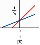
The lineweaver-Burk equation for the uncompetitive inhibition is, \(\frac{1}{v_{0}}=\left(\frac{K_{m}}{V_{\max }}\right) \frac{1}{[s]}+\frac{\alpha^{\prime}}{V_{\max }}\)

The corresponding lineweaver-Burk plot for the uncompetitive inhibition is shown below:

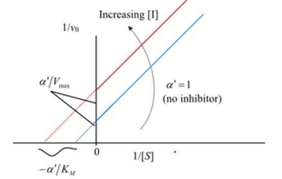
Plot 3: Lineweaver-Burk plot in the presence of the uncompetitive inhibitor

Compare the specified plot with the plot-3. Thus, based on the plot the enzyme reaction is an uncompetitive inhibition type.

 

Part-F

Compare the specified plot with plot-3, Thus, the blue line indicates the line equation without inhibitor and, the red line indicates the line equation with inhibitor.