Question

Questions 28-35 are related to the following The following table is the regression summary output for a model depicting the impact of years of schooling (EDUCTION) on hourly wage rate (WAGE). SUMMARY OUTPUT Regression Statistics Multiple R 0.47100 R Square Adjusted R Square 0.22106 Standard Error Observations 1000 ANOVA df SS MS F Significance F Regression 1 284.5202001 2.3433E-56 Residual 142.4243578 Total 999 182662.1158 Coefficients Std Error t Stat P-value Lower 95% Upper 95% Intercept 1.6551 -3.8378 0.0001 -9.6000 -3.1041 EDUCATION 0.0000 Use the following calculations first: ∑xy = 310428.68 x = EDUCATION n = 1000 y = WAGE x̅ = 13.907 y̅ = 20.83103 ∑x² = 204011 28 The model predicts that wage rises by _______ for each additional year of schooling. a $2.16 b $2.11 c $2.05 d $1.95 29 The predicted WAGE for 16 years of schooling is, a $26.44 26.44 b $25.67 25.67 c $24.92 24.92 d $23.93 23.93 30 SSE = ______ a 142139.51 b 140718.11 c 139310.93 d 137917.82 31 The measure of closeness of fit, or measure of dispersion of observed expenditure on food around the regression line is, a 10.24 b 11.93 c 12.12 d 12.85 32 The fraction of the variations in WAGE explained by years of schooling is, a 0.2218 b 0.2440 c 0.2562 d 0.2690 33 se(b₁) = ______ a 0.312 b 0.225 c 0.198 d 0.116 34 The test statistic to test the hypothesis that years of schooling has no impact on wage is, a 18.227 b 16.868 c 14.645 d 9.936 35 The upper end of the 95% interval estimate for the population slope parameter is, a 3.16 b 2.95 c 2.18 d 1.88

Answer 1

Given that y=wage (hourly wage) and x is education (years of schooling)

the model that we want to estimate is

where is the intercept of regression line

is the slope of regression line

is a random disturbance

We will first estimate the coefficients

the estimated regression equation is

28) The slope coefficient of education is 1.9546. This indicates that for each additional year of education, the wage increases by $1.9546

ans: d) $1.95

29) The predicted WAGE for 16 years of schooling is got by substituting x=16 in the estimated regression line

ans: c) The predicted WAGE for 16 years of schooling is $24.92

30) From the table we have the value of MSE (mean square error/residual)

MSE=142.42436

The degrees of freedom for SSE (sum of square Errors/residuals) is n-k-1 = 1000-1-1 =998 (where k=1 is the number of independent variables)

We can get SSE using

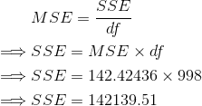
ans: a) 142139.51

31) Standard error of regression is a measure of closeness of fit, or measure or dispersion of wages around the regression line

The standard error is calculated as

ans: b) 11.93

32) the value of R-Square indicates the fraction of the variations in wage explained by years of schooling

We can calculate R2 using

We can also calculate this as

ans: a: 0.2218

33) The standard error of the estimate of is given by

ans: d) 0.116

34) Years of schooling would have no impact on wages if the coefficient of wage is equal to zero.

That means we want to test the following hypotheses

this means the the hypothesized value of the slope coefficient is

the test statistics is

ans: b) 16.868

35) 95% confidence interval indicates that the level of significance is .

The critical value of t is obtained for for a degrees of freedom = n-k-1=1000-1-1=998

From the t tables we can get an approximate value of

The 95% confidence interval is

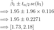
the upper end of the 95% interval estimate for the population parameter is ans: c) 2.18

the lower end of the 95% interval estimate for the population parameter is ans: 1.73