Question

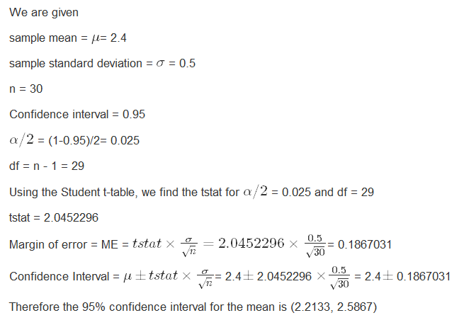
. A photocopier company claims that the average time it takes its technicians to service its brand of photocopiers onsite is two hours. To test this claim, 30 service times are recorded. The sample mean of the service times was 2.4 hours and the sample standard deviation was 0.5 hours. For µ denoting the mean service time, the hypotheses to be tested are: H0 : µ = 2 versus H1 : µ ̸= 2.

(a) Using the fact that t29,0.975 = 2.045, calculate a 95% confidence interval for the mean service time assuming that service time is normally distributed.

(b) Does your interval provide evidence that the company’s claim is false? That is, do you reject H0? Explain.

(c) Write a simple statement that summarises your findings.

2. A quality control inspector is interested in comparing two concreting companies with respect to overall quality of their work. One measure of quality is whether or not the concrete that has been poured is at least 15 centimeters (cm) thick. The inspector has recorded details for jobs from both companies and is now interested in whether the companies differ with respect to this measure of quality. Let p1 denote the true proportion of times that Company 1 will fail to pour concrete at least 15 cm thick and similarly let p2 denote the proportion for Company 2. The data collected for Company 1 shows that out of 120 jobs measured, 14 of these were less than 15 cm thick. For Company 2, 21 jobs out of 85 resulted in concrete less than 15 cm thick.

(a) Carry out a hypothesis test comparing the two proportions by using the R function prop.test. From the R output find and report the following: i. The estimates to p1 and p2. ii. The approximate 95% confidence interval for p1 − p2. iii. The p-value for the test comparing p1 and p2.

(b) Using the p-value you reported above, can you reject that the proportions are equal at the α = 0.05 significance level? Explain.

(c) Does your confidence interval suggest that one company performs better than the other with respect to this measure of quality? If so, which company performs better and why? If not then clearly explain why this is the case.

(d) Provide a simple statement that summarises the findings you have reported above.

3. Suppose that the scientists are concerned with the growth of the orange trees in their area. Load the data called ‘Orange’ (the Excel copy is saved in datasets folder in LMS) in R. Throughout we will assume that the data is stored in R as the data frame Orange. This dataset consists of three variables; Soil (soil enzymes level) , age (days since 31/12/1968) and the circumference (diameter of the trunk of the tree).

(a) To visualize any linear relationship between the dependent (response) variable Circumference and independent (predictor) variables Soil and Age, create two separate (one for each predictor) scatter plots with a smooth line, utilizing the ‘scatter.smooth’ command.

(b) In order to check for outliers, produce three BoxPlots of the variables Age, Soil and Circumference, by dividing the graph area into three columns, using the command ‘mfrow’. 1 (c) Execute the following command to obtain least squares estimates and associated output in R. lm.model <- lm(Circumference ~ Age + Soil, data = Orange) summary(lm.model) Provide a copy of your results displayed by summary(lm.model).

(d) Create plots of the residual versus fits and the Q-Q plot of the standardised residuals. Do you think the residuals versus fits plot or the Q-Q plot of the residuals suggest that there are any linear regression model violations that we need to be concerned with? Justify your answer with reference to both of the plots. NOTE: Regardless of your answer to (d), for the remainder of this question please assume that there are no linear regression model violations. (e) Does the R output suggest that the regression model fits the data well? Explain. (f) What are the estimates of the coefficients for the Age and Soil explanatory variables? Interpret these estimated coefficients. (g) Let β1 denote the true coefficient for the Age explanatory variable and consider the hypotheses H0 : β1 = 0 versus H1 : β1 ̸= 0. Do you reject the null hypothesis at the α = 0.05 significance level? Explain. (h) Repeat (g), but this time for the coefficient for the Soil explanatory variable. You may denote this coefficient as β2. (i) Using the fact that t32,0.975 = 2.037, construct 95% confidence interval for β1. (j) For a soil enzymes level of 2 and age of 500, what is the estimated circumference measurement from your model? (k) For a soil enzymes level of 2 and age of 500 that you considered above, provide a 95% confidence interval and 95% prediction interval for the circumference of the tree. Provide a justification as to why these intervals are different (i.e. what are these intervals used for?).

Answer 1

Question 1 (solved)

(a) Using the fact that t29,0.975 = 2.045, calculate a 95% confidence interval for the mean service time assuming that service time is normally distributed.

(b) Does your interval provide evidence that the company’s claim is false? That is, do you reject H0? Explain.

Yes, Ho is rejected, since the confidence interval (2.2133, 2.5867) does not contain 2.

(c) Write a simple statement that summarises your findings.

From the 95% confidence interval, we have sufficient evidence to conclude that the mean service time is different than 2.