Question

Problem 4: House Prices

Use the “Fairfax City Home Sales” dataset for parts of this problem.

a) Use StatCrunch to construct an appropriately titled and labeled relative frequency histogram of Fairfax home closing prices stored in the “Price” variable. Copy your histogram into your document.

b) What is the shape of this distribution? Answer this question in one complete sentence.

c) Assuming the population has a similar shape as the sample with population mean $510,000 and population standard deviation $145,000; calculate the probability that in a random sample of size 10, the mean of the sample will be greater than $600,000. You may assume a random sample was taken and the sample came from a big population. However, be sure to check the central limit theorem condition of a large sample size before completing this problem using one complete sentence. If this condition is not met, you cannot complete the problem.

d) Assuming the population has a similar shape as the sample with population mean $510,000 and population standard deviation $145,000; calculate the probability that in a random sample of size 36, the mean of the sample will be greater than $600,000. You may assume a random sample was taken and the sample came from a big population. However, be sure to check the central limit theorem condition of a large sample size before completing this problem using one complete sentence. If this condition is not met, you cannot complete the problem.

Data:

Price Year, Days, TLArea, Acres

369900   1922   44   1870   0.39

373000   1952   0   1242   0.27

375000   1952   8   932   0.15

375000   1950   2   768   0.19

379000   1952   31   816   0.21

380000   1941   53   1092   0.19

385000   1951   5   984   0.27

387700   1953   5   975   0.36

395000   1954   18   957   0.29

395000   1951   12   1105   0.22

399900   1954   29   1206   0.28

399900   1951   6   1226   0.18

400000   1954   31   957   0.27

410000   1949   6   1440   0.2

410000   1954   17   1344   0.23

412500   1954   4   1008   0.25

415000   1953   17   1371   0.28

420000   1954   2   957   0.25

426000   1952   3   1694   0.25

430000   1953   19   975   0.23

434900   1950   5   1128   0.18

435000   1954   32   1252   0.24

440000   1960   3   1161   0.26

440000   1954   2   1036   0.28

440000   1955   12   1645   0.28

440000   1960   5   1746   0.31

441000   1952   133   1062   0.23

442000   1961   4   1414   0.32

443000   1951   26   962   0.2

444900   1955   4   1122   0.19

446500   1953   3   962   0.26

450000   1952   2   1488   0.15

450000   1955   49   1122   0.23

450000   1979   0   1092   0.28

450000   1951   70   962   0.2

450000   1957   23   1300   0.51

451000   1947   12   1325   0.34

455000   1952   7   2267   0.81

455000   1962   4   1050   0.31

460000   1955   5   997   0.3

460000   1954   10   1125   0.17

465000   1954   77   1288   0.46

465900   1947   21   1309   0.19

469000   1963   153   1149   0.27

474000   1959   5   1319   0.32

475000   1955   4   1530   0.28

475000   1953   29   1008   0.2

475000   1955   6   1530   0.28

475000   1956   116   1345   0.5

475000   1956   1   1530   0.28

480000   1960   27   1236   0.27

480000   1959   133   1527   0.24

485000   1955   4   1008   0.24

485000   1956   74   977   0.24

488000   1960   11   1972   0.33

500000   1963   0   2145   0.25

500000   1953   14   1758   0.54

500500   1955   6   1630   0.28

510000   1959   5   1680   0.34

512000   1963   0   1968   0.22

519000   1961   1   1312   0.29

520000   1954   15   1492   0.25

520000   1958   80   1443   0.33

520000   1963   122   1822   0.32

530000   1962   6   1393   0.29

540000   1962   12   1414   0.25

543600   1962   4   1414   0.24

560000   1967   5   1530   0.28

560000   1961   16   1438   0.53

565000   1947   6   1510   0.25

565500   1967   5   1217   0.26

589000   1954   32   2368   0.3

593000   1954   9   2044   0.25

610000   1978   140   2091   0.09

655000   1976   180   2728   0.24

660000   1947   10   2635   0.22

665000   1950   37   2645   0.57

685000   1982   120   2752   0.09

795000   2002   259   3402   0.12

852000   2000   4   3215   0.11

895000   2000   63   3230   0.11

930000   2015   135   3175   0.15

940000   1860   42   3038   0.57

968500   1850   74   3630   0.34

1100000   2004   161   3640   0.19

Answer 1

(a) The Histogram is obtained as:

> price = c(369900, 373000, 375000, 375000, 379000, 380000, 385000, 387700, 395000, 395000, 399900, 399900, 400000, 410000, 410000, 412500, 415000, 420000, 426000, 430000, 434900, 435000, 440000, 440000, 440000, 440000, 441000, 442000, 443000, 444900, 446500, 450000, 450000, 450000, 450000, 450000, 451000, 455000, 455000, 460000, 460000, 465000, 465900, 469000, 474000, 475000, 475000, 475000, 475000, 475000, 480000, 480000, 485000, 485000, 488000, 500000, 500000, 500500, 510000, 512000, 519000, 520000, 520000, 520000, 530000, 540000, 543600, 560000, 560000, 565000, 565500, 589000, 593000, 610000, 655000, 660000, 665000, 685000, 795000, 852000, 895000, 930000, 940000, 968500, 1100000)

> hist(price, breaks = 10, main="Fairfax Home Closing Prices", xaxt='n')

> axis(side=1, at=seq(350000,1500000, 100000), labels=seq(350000,1500000, 100000))

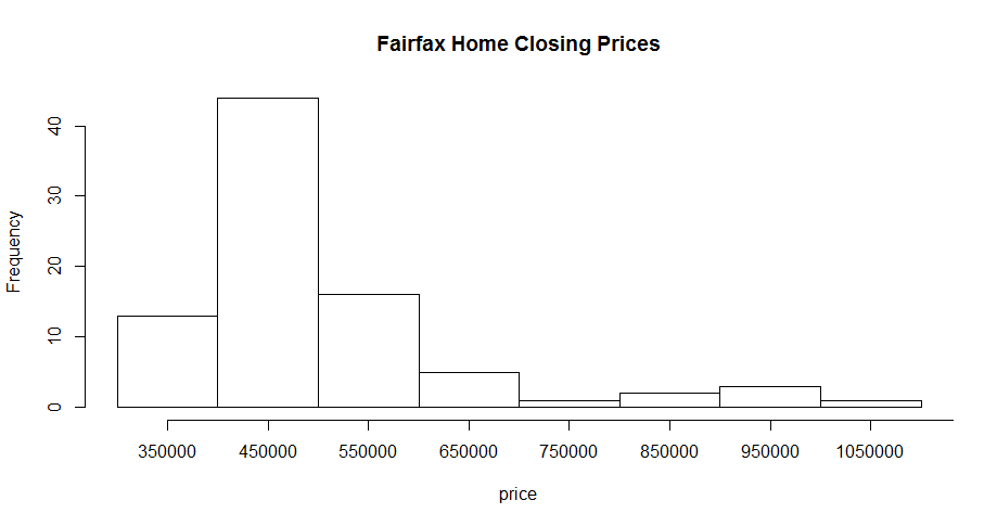
(b) The Histogram is skewed (Non-Normal) to the right, which the tail is on the right side.

(c) We are to obtain:

where is the sample mean.

Thus, the probability that in a random sample of size 10, the mean of the sample will be greater than $600,000 is obtained as 0.02483511.

(d) We are to obtain:

where is the sample mean.

Thus, the probability that in a random sample of size 36, the mean of the sample will be greater than $600,000 is obtained as 0.06602641.