Question

Q3. Hypothesis: Informing people about recycling causes them to recycle more.

Study design: 50 households were randomly assigned to a treatment group where they were

informed by letter about proper recycling habits and its benefit on environment, while 50

different households were randomly assigned to a control group that did not receive such a letter.

After 3 months, the weekly average recycling amount in the treatment group was 12.4 lbs (

sd

=

2.5), while the weekly average recycling amount in the control group was 3.7 lbs (

sd

= 1.1)

d. Determine the appropriate test: z-test or t-test. Explain why you chose that test.

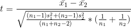
e. Calculate the appropriate test statistic

f. Decide whether you should reject the null hypothesis.

Answer 1

Q3. Hypothesis: Informing people about recycling causes them to recycle more.

Study design: 50 households were randomly assigned to a treatment group where they were

informed by letter about proper recycling habits and its benefit on environment, while 50

different households were randomly assigned to a control group that did not receive such a letter.

After 3 months, the weekly average recycling amount in the treatment group was 12.4 lbs (sd=2.5), while the weekly average recycling amount in the control group was 3.7 lbs (sd= 1.1)

d. Determine the appropriate test: z-test or t-test. Explain why you chose that test.

T test is used because population standard deviation is not known.

Two sample t test

Ho: µ1 = µ2   H1: µ1 > µ2

Upper tail t test

e. Calculate the appropriate test statistic

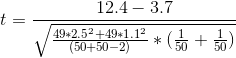
t=22.5234

f. Decide whether you should reject the null hypothesis.

DF = n₁+n₂-2 =98

Table value of t with 98 DF at 0.05 level = 1.6606

Rejection Region: Reject Ho if or t > 1.6606

Calculated t = 22.5234 falls in the rejection region

The null hypothesis is rejected.

We conclude that informing people about recycling causes them to recycle more.

Pooled-Variance t Test for the Difference Between Two Means
(assumes equal population variances)
Data
Hypothesized Difference	0
Level of Significance	0.05
Population 1 Sample
Sample Size	50
Sample Mean	12.4
Sample Standard Deviation	2.5
Population 2 Sample
Sample Size	50
Sample Mean	3.7
Sample Standard Deviation	1.1
Intermediate Calculations
Population 1 Sample Degrees of Freedom	49
Population 2 Sample Degrees of Freedom	49
Total Degrees of Freedom	98
Pooled Variance	3.7300
Standard Error	0.3863
Difference in Sample Means	8.7000
t Test Statistic	22.5234
Upper-Tail Test
Upper Critical Value	1.6606
p-Value	0.0000
Reject the null hypothesis