Questions
What are the leakages and injections in the scenario from #1 and what equation holds between...
- What are the leakages and injections in the scenario from #1 and what equation holds between them in equilibrium?
Injections
in the circular flow of income, spending which is not generated by
households, examples are investments, government spending and
exports.
Leakages
or withdrawals in the circular flow of income, spending by
households which does not flow back into the domestic firms,
examples are savings, taxes and imports.
In: Economics
Write a one page summary on Minutes of the Federal Open Market Committee Staff Economic Outlook...
Write a one page summary on Minutes of the Federal Open Market Committee
Staff Economic Outlook
The staff projection for U.S. economic activity prepared for the
March FOMC meeting was somewhat stronger, on balance, than the
forecast at the time of the January meeting. The near-term forecast
for real GDP growth was revised down a little; the incoming
spending data were a bit softer than the staff had expected, and
the staff judged that the softness was not associated with residual
seasonality in the data. However, the slowing in the pace of
spending in the first quarter was expected to be transitory, and
the medium-term projection for GDP growth was revised up modestly,
largely reflecting the expected boost to GDP from the federal
budget agreement enacted in February. Real GDP was projected to
increase at a faster pace than potential output through 2020. The
unemployment rate was projected to decline further over the next
few years and to continue to run below the staff's estimate of its
longer-run natural rate over this period.
The projection for inflation over the medium term was revised up a bit, reflecting the slightly tighter resource utilization in the new forecast. The rates of both total and core PCE price inflation were projected to be faster in 2018 than in 2017. The staff projected that inflation would reach the Committee's 2 percent objective in 2019.
The staff viewed the uncertainty around its projections for real GDP growth, the unemployment rate, and inflation as similar to the average of the past 20 years. The staff saw the risks to the forecasts for real GDP growth and the unemployment rate as balanced. On the upside, recent fiscal policy changes could lead to a greater expansion in economic activity over the next few years than the staff projected. On the downside, those fiscal policy changes could yield less impetus to the economy than the staff expected if the economy was already operating above its potential level and resource utilization continued to tighten, as the staff projected. Risks to the inflation projection also were seen as balanced. An upside risk was that inflation could increase more than expected in an economy that was projected to move further above its potential. Downside risks included the possibilities that longer-term inflation expectations may have edged lower or that the run of low core inflation readings last year could prove to be more persistent than the staff expected.
In: Economics
Albright Chemical Company currently operates three manufacturing plants inColorado, Utah, and Arizona. Annual carbon emissions for...
Albright Chemical Company currently operates three manufacturing plants inColorado, Utah, and Arizona. Annual carbon emissions for these plants in the first quarter of 2018 are120,000metric tons per quarter (or 480,000 metric tons in 2018). Albright management is investigating improved manufacturing techniques that will reduce annual carbon emissions to below 456,000metric tons so that the company can meet Environmental Protection Agency guidelines by 2019. Costs and benefits are as follows: Total cost to reduce carbon emissions $9 per metric ton reduced in 2019 below 480,000 metric tons Fine in 2019 if EPA guidelines are not met $423,000 Albright Management has chosen to use Kaizen budgeting to achieve its goal for carbon emissions. 1. If Albright reduces emissions by 2 % each quarter, beginning with the second quarter of 2018, will the company reach its goal of 456,000 metric tons by the end of 2019? 2. What would be the net financial cost or benefit of their plan? Ignore the time value of money. 3. What factors other than cost might weigh into Albright's decision to carry out this plan? Requirement 1. If Albright reduces emissions by 2 % each quarter, beginning with the second quarter of 2018, will the company reach its goal of 456,000 metric tons by the end of 2019? (Round all intermediary calculations and the amounts you input in the cells to the nearest dollar.) Begin by calculating the quarterly emissions for each quarter through the end of 2019. Quarterly emissions Quarter (metric tons) 2018 Q1 2018 Q2 2018 Q3 2018 Q4 2019 Q1 2019 Q2 2019 Q3 2019 Q4 Will the company reach its goal of 456,000 metric tons by the end of 2019? Yes, Albright will / No, Albright will not reach its goal of 456,000 metric tons by the end of 2019. Requirement 2. What would be the net financial cost or benefit of their plan? Ignore the time value of money. (Use parentheses or a minus sign to show a net benefit.) _______________ _______________ _______________ ________________ Net cost (benefit) of plan _________________ Requirement 3. What factors other than cost might weigh into Albright's decision to carry out this plan? Avoidance of the EPA fine should / should not be the company's sole motivation in carrying out this plan. Reducing carbon emissions has no impact on the environment is good for the environment, and will contribute to a smaller impact on climate change / is too costly and may not contribute to a smaller impact on climate change. Albright may be able to share this plan with the public to gain favorable publicity / petition the EPA for a waiver. Albright could choose to end this plan at the end of 2019, and still avoid the EPA fine / pay the EPA fine; however, company management has no obligation to reduce carbon emissions should / strive to continue reducing carbon emissions if they have the technology to do so.
In: Accounting
6. Industries whose firms have downward-sloping LRAC curves that reach the minimum efficient scale at large values...
6. Industries whose firms have downward-sloping LRAC curves that reach the minimum efficient scale at large values of output relative to the size of the market:
a. Tend to have a large number of small firms.
b. Tend to have a small number of large firms.
c. Tend to have a wide range of firm sizes.
d. Tend to have a few large firms and a few small ones.
7. The Average/Marginal Rule says that
a. When MC is above ATC, ATC must be falling.
b. When MC is falling, ATC must be falling.
c. When MC is below AFC, AFC must be rising.
d. None of the above.
8. The perfect substitutes model in production has:
a. Conventional isoquants
b. Linear isoquants.
c. L- shaped isoquants.
d. Backward-bending isoquants.
9. The main point of Frank’s Cullen Gates story is:
a. Gates should move his miniature golf course to Manhattan.
b. Accounting and economic profits are the same.
c. Firm decisions should be made on the basis of economic profits.
d. Firm decisions should be made on the basis of accounting profits.
10. The main point of Frank’s “An Efficient Manager” story is:
a. Efficient managers lower costs for their firms.
b. Firms with efficient managers will have lower costs in the long run.
c. Efficient managers will be paid more.
d. In the long run, firms with and without efficient managers will earn the same profits.
In: Economics
3. Saving and net flows of capital and goods In a closed economy, saving and gross...
3. Saving and net flows of capital and goods
In a closed economy, saving and gross investment must be equal, but this is not the case in an open economy. In the following problem, you will explore how saving and gross investment are connected to the international flow of capital and goods in an economy. Before delving into the relationship between these various components of an economy, you will be asked to recall some relationships between aggregate variables that will be useful in your analysis.
Recall the components that make up GDP. National income (Y) equals total expenditure on the economy’s output of goods and services. Thus, where C = consumption, I = gross investment, G = government spending, and NX = net exports, Y is defined as follows:
Y = (C - I + G + NX) / (C + I + G - NX) / (C + I + G + NX) / C + I - G - NX) PICK ONE
National saving (S) is the income of the nation that is left after paying for government spending and consumption. Therefore, S is defined as follows:
S = (Y - C) / (Y - I - C) / (Y - C - G) / (Y - I) PICK ONE
Rearranging the previous equation and solving for Y yields Y = (S + I) / (S + I + C) / (S + C + G) / (S + C) PICK ONE
Plugging this into the original equation showing the various components of income results in the following relationship:
S = (I + G + NX) / (I + NX) / (C + G + NX) / (G + NX) PICK ONE
This is equivalent to S = (G + NCO) / (C + G + NCO) / (I + NCO) / (I + G + NCO) PICK ONE
since net exports must equal net capital outflow (NCO, also known as net foreign investment).
Now suppose that a country is experiencing a trade deficit. Determine the relationships between the entries in the following table and enter these relationships using the following symbols: > (greater than), < (less than), or = (equal to).
Outcomes of a trade deficit [pick one for each bracket]
Net Exports [ < , = , >] 0
Imports [ <, =, >] Exports
C + I + G [<, =, >] Y
Gross Investment [<, =, >] Saving
0 [<, =, >] Net Capital Outflow
In: Economics
Baggy Company has the following information related to the production of handbags for the 2nd quarter...
Baggy Company has the following information related to the production of handbags for the 2nd quarter of 2017:
• Budgeted sales volume April 150 bags • Budgeted sales volume May 175 bags • Budgeted sales volume June 160 bags • Selling price per bag $45 • Cost of leather per yard $7 • Leather per bag 1.5 yards • Cost of direct labor per hour $10 • Direct labor per bag 0.5 hour • Manufacturing overhead cost per bag $5.50 • Desired ending inventory for bags is 20% of current month’s sales units • Desired ending inventory for leather is 10% of current month’s Direct material yards required for production • Ending inventory of leather at March 31 was 18 yards (use as Beginning inventory for April) • Ending inventory of bags at March 31 was 25 bags (use as Beginning inventory for April) • Variable selling and admin cost per bag $5 • Fixed selling and admin cost per month $1,550 • Income tax rate $25%
• Using the data above, put together the Master Budget (use the format provided on page 2 of instructions) in Excel from a new workbook for Baggy Company – include:
o Sales Budget (for April, May, June and the entire 2nd quarter of 2017) o Production Budget (for April, May, June and the entire 2nd quarter of 2017) o Direct Materials Budget (for April, May, June and the entire 2nd quarter of 2017) o Direct Labor Budget (for April, May, June and the entire 2nd quarter of 2017) o Budgeted Income Statement (for 2nd Quarter only) ? First sheet of workbook should contain data section ? Set up each budget in its own worksheet and link cells to data sheet or to previous budget where appropriate (Example: Budgeted Sales Units from Sales Budget should be linked to Production Budget) ? All numbers should have appropriate formatting o Data sheet and all budgets should be set up so that one change to the data section will automatically recalculate Net Income • Format each worksheet to be visually organized and appealing and print to one page • Add your name to the bottom right-hand footer of each sheet • Rename your completed Excel file to include your first initial and last name at the end of the file name (example: Acc 255 Graded Assignment #10 L. Akeo) • Submit your completed Excel file back to the Assignment in Laulima by the due date indicated in the assignment.
Grading Rubric Requirements Maximum Points Budgets are in good form 10 Budget totals are accurately calculated using appropriate formulas in Excel 15 All sheets are linked from data sheet to Income Statement 15 Each sheet prints to one page and is visually organized and appealing 5 Add your name to each footer and to file name 5 Total points 50 Sales budget Budgeted sales units x selling price per bag = Total budgeted sales dollars Hint: Total sales for the entire 2nd quarter should come out to $21,825. Production Budget Budgeted sales units + Desired ending inventory of bags (20% of current months’ sales units) (-) Beginning inventory (20% of last month’s sales units) = Required production units (bags) Hint: Required production units for the entire 2nd quarter should come out to 492 units (bags). Direct Materials Budget Required production units (bags) x Direct material yards per bag = Direct material yards required for production + Desired ending inventory (10% of current month’s Direct material yards required for production) (-) Beginning inventory (10% of last month’s Direct material yards required for production) = Required purchases of direct material yards x Material cost per yard = Total cost of direct material purchases Hint: Total cost of direct material purchases for the entire 2nd quarter should come out to $5,204.85. Direct Labor Budget Required production units x DL hours per bag Required DL hours x Standard DL cost per hour Total DL cost
Hint: Total direct labor cost for the entire 2nd quarter should come out to $2,460. Budgeted Income Statement Total sales Less: COGS [(Total cost per unit* x total units sold for the quarter) = Gross profit Less: Selling and admin (Variable cost per bag x total bags sold) + Fixed costs for the quarter = Income before taxes Less: Income tax expense = Net income *To get Total cost per unit = [(Cost of leather per yd x yds needed per bag) + (DL cost per hr x DL hrs per bag) + Manufacturing OH cost per bag] Hint: Net income should come out to $3,423.75.
In: Accounting
Based upon the preceding data, would you expect the ending inventory using the last-in, first-out method to be higher or lower?
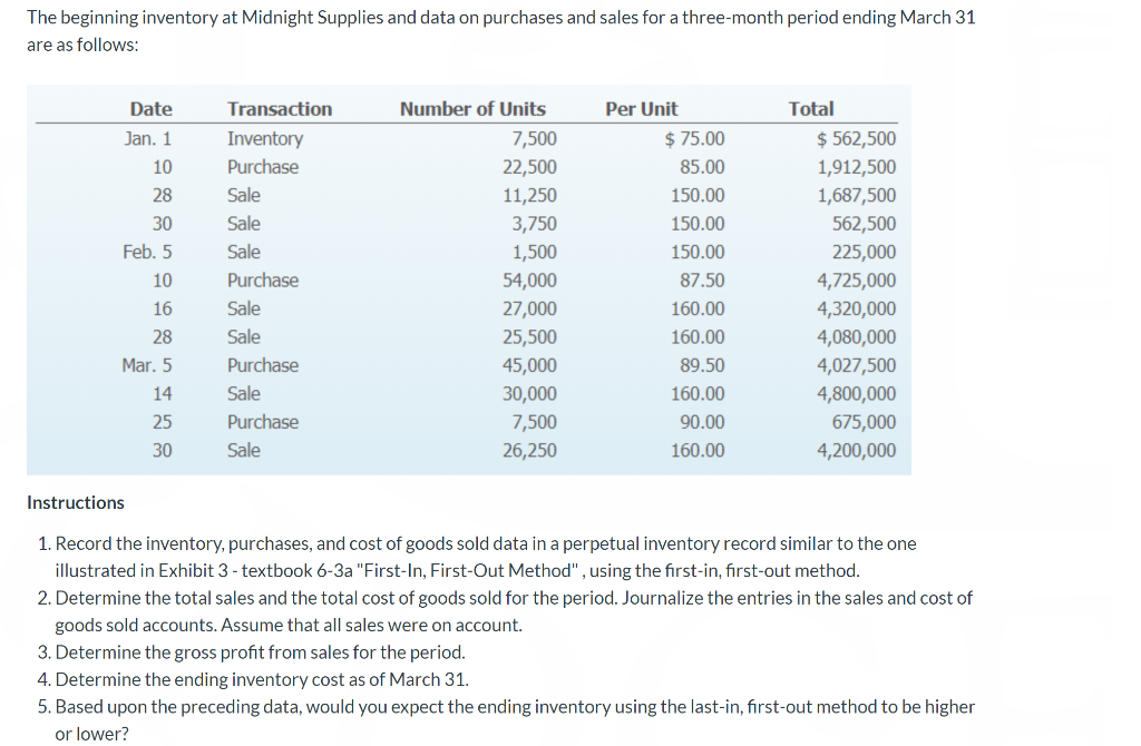
The beginning inventory at Midnight Supplies and data on purchases and sales for a three-month period ending March 31 are as follows:
| Date | Transaction | Number of Units | Per Unit | Total | ||||
|---|---|---|---|---|---|---|---|---|
| Jan. 1 | Inventory | 7,500 | $75.00 | $562,500 | ||||
| 10 | Purchase | 22,500 | 85.00 | 1,912,500 | ||||
| 28 | Sale | 11,250 | 150.00 | 1,687,500 | ||||
| 30 | Sale | 3,750 | 150.00 | 562,500 | ||||
| Feb. 5 | Sale | 1,500 | 150.00 | 225,000 | ||||
| 10 | Purchase | 54,000 | 87.50 | 4,725,000 | ||||
| 16 | Sale | 27,000 | 160.00 | 4,320,000 | ||||
| 28 | Sale | 25,500 | 160.00 | 4,080,000 | ||||
| Mar. 5 | Purchase | 45,000 | 89.50 | 4,027,500 | ||||
| 14 | Sale | 30,000 | 160.00 | 4,800,000 | ||||
| 25 | Purchase | 7,500 | 90.00 | 675,000 | ||||
| 30 | Sale | 26,250 | 160.00 | 4,200,000 | ||||
Instructions
1. Record the inventory, purchases, and cost of goods sold data in a perpetual inventory record similar to the one illustrated in Exhibit 3 - textbook 6-3a "First-In, First-Out Method", using the first-in, first-out method.
2. Determine the total sales and the total cost of goods sold for the period. Journalize the entries in the sales and cost of goods sold accounts. Assume that all sales were on account.
3. Determine the gross profit from sales for the period.
4. Determine the ending inventory cost as of March 31.
5. Based upon the preceding data, would you expect the ending inventory using the last-in, first-out method to be higher or lower?
In: Accounting
The beginning inventory for Dunne Co. and data on purchases and sales for a three-month period...
The beginning inventory for Dunne Co. and data on purchases and
sales for a three-month period are as follows:
| Date | Transaction | Number of Units |
Per Unit | Total | ||
|---|---|---|---|---|---|---|
| Apr. 3 | Inventory | 25 | $1,200 | $30,000 | ||
| 8 | Purchase | 75 | 1,240 | 93,000 | ||
| 11 | Sale | 40 | 2,000 | 80,000 | ||
| 30 | Sale | 30 | 2,000 | 60,000 | ||
| May 8 | Purchase | 60 | 1,260 | 75,600 | ||
| 10 | Sale | 50 | 2,000 | 100,000 | ||
| 19 | Sale | 20 | 2,000 | 40,000 | ||
| 28 | Purchase | 80 | 1,260 | 100,800 | ||
| June 5 | Sale | 40 | 2,250 | 90,000 | ||
| 16 | Sale | 25 | 2,250 | 56,250 | ||
| 21 | Purchase | 35 | 1,264 | 44,240 | ||
| 28 | Sale | 44 | 2,250 | 99,000 | ||
Required:
1. Determine the inventory on June 30 and the cost of goods sold for the three-month period, using the first-in, first-out method and the periodic inventory system. Round the weighted average unit cost to the nearest cent.
| Inventory, June 30 | $ |
| Cost of goods sold | $ |
2. Determine the inventory on June 30 and the cost of goods sold for the three-month period, using the last-in, first-out method and the periodic inventory system.
| Inventory, June 30 | $ |
| Cost of goods sold | $ |
3. Determine the inventory on June 30 and the cost of goods sold for the three-month period, using the weighted average cost method and the periodic inventory system.
Note: Round the weighted average unit cost to the nearest dollar and final answers to the nearest dollar.
| Inventory, June 30 | $ |
| Cost of goods sold | $ |
4. Compare the gross profit and June 30 inventories using the following column headings. Enter all amounts as positive numbers.
| FIFO | LIFO | Weighted Average | |
|---|---|---|---|
| Sales | $ | $ | $ |
| Cost of goods sold | |||
| Gross profit | $ | $ | $ |
| Inventory, June 30 | $ | $ | $ |
In: Accounting
Periodic Inventory by Three Methods The beginning inventory for Dunne Co. and data on purchases and...
Periodic Inventory by Three Methods
The beginning inventory for Dunne Co. and data on purchases and
sales for a three-month period are as follows:
| Date | Transaction | Number of Units |
Per Unit | Total | ||
|---|---|---|---|---|---|---|
| Apr. 3 | Inventory | 25 | $1,200 | $30,000 | ||
| 8 | Purchase | 75 | 1,240 | 93,000 | ||
| 11 | Sale | 40 | 2,000 | 80,000 | ||
| 30 | Sale | 30 | 2,000 | 60,000 | ||
| May 8 | Purchase | 60 | 1,260 | 75,600 | ||
| 10 | Sale | 50 | 2,000 | 100,000 | ||
| 19 | Sale | 20 | 2,000 | 40,000 | ||
| 28 | Purchase | 80 | 1,260 | 100,800 | ||
| June 5 | Sale | 40 | 2,250 | 90,000 | ||
| 16 | Sale | 25 | 2,250 | 56,250 | ||
| 21 | Purchase | 35 | 1,264 | 44,240 | ||
| 28 | Sale | 44 | 2,250 | 99,000 | ||
Required:
1. Determine the inventory on June 30 and the cost of goods sold for the three-month period, using the first-in, first-out method and the periodic inventory system. Round the weighted average unit cost to the nearest cent.
| Inventory, June 30 | $ |
| Cost of goods sold | $ |
2. Determine the inventory on June 30 and the cost of goods sold for the three-month period, using the last-in, first-out method and the periodic inventory system.
| Inventory, June 30 | $ |
| Cost of goods sold | $ |
3. Determine the inventory on June 30 and the cost of goods sold for the three-month period, using the weighted average cost method and the periodic inventory system.
Note: Round the weighted average unit cost to the nearest dollar and final answers to the nearest dollar.
| Inventory, June 30 | $ |
| Cost of goods sold | $ |
4. Compare the gross profit and June 30 inventories using the following column headings. Enter all amounts as positive numbers.
| FIFO | LIFO | Weighted Average | |
|---|---|---|---|
| Sales | $ | $ | $ |
| Cost of goods sold | |||
| Gross profit | $ | $ | $ |
| Inventory, June 30 | $ | $ | $ |
In: Accounting
Periodic inventory by three methods The beginning inventory for Midnight Supplies and data on purchases and...
Periodic inventory by three methods
The beginning inventory for Midnight Supplies and data on purchases and sales for a three-month period are shown below:
| Date | Transaction | Number of Units |
Per Unit | Total | ||
| Jan. 1 | Inventory | 7,500 | $75.00 | $562,500 | ||
| 10 | Purchase | 22,500 | 85.00 | 1,912,500 | ||
| 28 | Sale | 11,250 | 150.00 | 1,687,500 | ||
| 30 | Sale | 3,750 | 150.00 | 562,500 | ||
| Feb. 5 | Sale | 1,500 | 150.00 | 225,000 | ||
| 10 | Purchase | 54,000 | 87.50 | 4,725,000 | ||
| 16 | Sale | 27,000 | 160.00 | 4,320,000 | ||
| 28 | Sale | 25,500 | 160.00 | 4,080,000 | ||
| Mar. 5 | Purchase | 45,000 | 89.50 | 4,027,500 | ||
| 14 | Sale | 30,000 | 160.00 | 4,800,000 | ||
| 25 | Purchase | 7,500 | 90.00 | 675,000 | ||
| 30 | Sale | 26,250 | 160.00 | 4,200,000 | ||
1. Determine the inventory on March 31 and the cost of goods sold for the three-month period, using the first-in, first-out method and the periodic inventory system.
| Inventory, March 31 | $ |
| Cost of goods sold | $ |
2. Determine the inventory on March 31 and the cost of goods sold for the three-month period, using the last-in, first-out method and the periodic inventory system.
| Inventory, March 31 | $ |
| Cost of goods sold | $ |
3. Determine the inventory on March 31 and the cost of goods sold for the three-month period, using the weighted average cost method and the periodic inventory system. Round the weighted average unit cost to the nearest cent.
| Inventory, March 31 | $ |
| Cost of goods sold | $ |
4. Compare the gross profit and the March 31 inventories, using the following column headings. For those boxes in which you must enter subtracted or negative numbers use a minus sign.
| FIFO | LIFO | Weighted Average | |
| Sales | $ | $ | $ |
| Cost of goods sold | |||
| Gross profit | $ | $ | $ |
| Inventory, March 31 | $ | $ | $ |
In: Accounting